Using R to work through Sokal and Rohlf's Biometry: Chapter 6 (The Normal Probability Distribution), sections 6.1-6.2

Previously in this series: Chapter 5 (Descriptive Statistics), section 5.5 and selected exercises.

Chapter 6 moves on from discrete distributions to the normal distribution,
#a continuous distribution that will be the basis of most statistics in the book.

Section 6.1 Frequency Distributions of Continuous Variables

A brief discussion of the section header's topic, nothing to code here.

Section 6.2 Properties of the Normal Distribution

#Let's check where it is.
?Distributions
?dnorm

#We can draw the normal distribution in a custom function as a plot using curve()
#and equation 6.1 on page 95.
normal.manual<-function(mean, sd){
curve((1/(sd*sqrt(2*pi)))*exp((-((x-mean)/sd)^2)/2),
      -4, 4, #go from -4 to +4 standard deviations.
      add = FALSE,
      ylab="freq",
      xlab="Y",
      type = "l")
}
normal.manual(0,1)

#You can get this automatically in R with dnorm.
curve(dnorm(x, mean=0, sd=1),
      -4, 4,
      col="white",
      lty="dashed",
      add=TRUE)
#I added a white dashed line over the original black line so you can see that they follow the same path.

#You can draw any of the distributions in Figure 6.2 using these functions
#(either the R one or the one we just made).

#Figure 6.3 shows the cumulative normal distribution function.

#Let's do that and then plot the normal probability density function on it.
#Cumulative first since that plot will go from 0 to 1.
curve(pnorm(x, mean=0, sd=1),
      -4, 4,
      lty="solid")

#Then add the normal probability density function (like the one we made earlier, just with the default line color).
curve(dnorm(x, mean=0, sd=1),
      -4, 4,
      lty="dashed",
      add=TRUE)

#To get out some of the values  shown in page 96, we use pnorm().
#http://stackoverflow.com/questions/34236648/r-function-to-calculate-area-under-the-normal-curve-between-adjacent-standard-de

pnorm(0, mean=0, sd=1)
#Just adding one value gives you a point estimate.
#50% will be found up to zero (the mean).

#The other values shown in Figure 6.3
pnorm(-1)
pnorm(-2)
#0 and 1 are the default values for mean and standard deviation, so you can leave them out if you want in this case.
#If you add more than one, it will tell you the values.
(pnorm(0:1))
#Use diff as suggested here to get the area under the curve.
diff(pnorm(0:1))
#This works because it uses the cumulative function to calculate it.
#If you go from -1 to 1 you can add them up to get the 68.27% shown under Figure 6.2 and on page 96.
sum(diff(pnorm(-1:1)))

#To go the other way, i.e. to see where 50% of the items fall, you have to use qnorm.
#Let's see what qnorm looks like.
curve(qnorm(x))
#It is essentially tipping Figure 6.3 on its side.
#The frequency is now x on the x-axis, and the standard deviations are the y axis.
#You can get the point values in Figure 6.3 this way:
qnorm(0.5)
qnorm(0.1587)
qnorm(0.0228)
#The last two are close with rounding since those values in Figure 6.3 were rounded.
#How to get the values on page 96, of where 50%, 95%, etc of items are found?
qnorm(0.5+0.5*0.5)
qnorm(0.95+0.5*0.05)
qnorm(0.99+0.5*0.01)
#The values that you input are not the percent values given on page 96.
#You put them in proportions (the quantile you want to get) PLUS
#half of the remaining value.
#If you put in 0.95, it will go from 0 to 0.95.  That isn't centered at the mean of 0,
#where the 50% quantile is.  There is 0.05 left at the end.  So we divide it by two
#to put it on either end.
#You would get the negative number for the standard deviation if you put in the opposite value.
qnorm(0.5*0.01)
#This also explains it nicely down where it starts talking about qnorm.
#https://cran.r-project.org/web/packages/tigerstats/vignettes/qnorm.html

#On pg. 98, they show calculation of standard deviates.
#This is described in such a way that they seem to be z scores although they are never named as such in the book.
#You can easily calculate this manually.
z.score<-function(x){
  (x-mean(x))/sd(x)
}

x<-c(1,2,3)
z.score(x)
#You can also use the scale() function.
#https://www.r-bloggers.com/r-tutorial-series-centering-variables-and-generating-z-scores-with-the-scale-function/

scale(x,
      center=TRUE,
      scale=TRUE)
#help notes that scale=TRUE divides by the standard deviation when
#center=TRUE, and center=TRUE substracts each number by the column mean.
#This is the same thing we did in the z-score function.

#Table 6.1 has expected frequencies for the normal distribution in column 2 for a sample of 1000 individuals.
#We can generate this with pnorm() and thinking about what the class marks mean.
#Because the class marks are separated by 0.5, we need to go 0.5 around each class mark and start at -5.25.
boundaries<-seq(from=-5.25,
                to=5.25,
                by=0.5)

pnorm.results<-pnorm(boundaries)
expected.freqs<-abs(diff(pnorm.results))
cbind(boundaries[-length(boundaries)]+0.25,
      #this takes the last entry off because we only need the lower bound for each class,
      #and adds 0.25 to get the class mark.
      round(expected.freqs*1000, 1))
#Then you can have a look at the table and see that it gives the same results as column 2 in Table 6.1.

Using R to work through Sokal and Rohlf's Biometry: Chapter 5 (Descriptive Statistics), section 5.4 and selected exercises

Previously in this series: Chapter 5 (Descriptive Statistics), section 5.3.

Section 5.4: Other Discrete Probability Distributions

?dhyper #hypergeometric
?dmultinom #multinomial
?dnbinom #negative binomial
#There are also options in various packages later for regression to use different distributions,
#although of these I've only ever used negative binomial.

#The logarithmic distribution requires an extra package.
#https://cran.r-project.org/web/views/Distributions.html
#extraDistr, VGAM, or gamlss.dst
#I installed extraDistr to test it out.
library(extraDistr)
?LogSeries
#and
?dlgser #The distributions in this package follow the same us of d, p, and q prefixes.

Exercises 5

#I'm doing the exercises that require new coding beyond what we have done already.

#Exercise 5.5
#The organism is present or absent in any given slide, assuming the person is diseased
#(if the person has the disease, their samples contain the organism but it's not very common).
#We want a false negative <1% of the time.  The organism is visible in 20% of the slides.
#At first I thought this was a Bayesian problem but I don't see how to do it that way.
#p=0.2 (organism visible), thus q=0.8 (organism present but not visible).
#We need to find the power of q=0.8 that equals 0.01 or smaller
#(1% false negative, which would be present but not visible).
#So, I made a while loop that cycled through to see how many times we need to raise 0.8
#to get to 0.01.  This explanation helped me figure out how to do this type of loop.

n<-0
i<-1
print(n)
while (i > 0.01) {
  print(i)
  print(n)
     i<-0.8^n
     n=n+1
}
#the last number printed is the number of slides needed.

Using R to work through Sokal and Rohlf's Biometry: Chapter 5 (Descriptive Statistics), section 5.3

Previously in this series: Chapter 5 (Introduction to Probability Distributions: Binomial and Poisson), sections 5.1-5.2.

Section 5.3: the Poisson distribution

?Distributions #Let's look in help again to find the Poisson distribution.
?dpois #We can see that R does similar calculations for Poisson in addition to the binomial distribution.

#To get column 3 (expected absolute frequencies) in table 5.5,
#there is the recursion formula given in equations 5.11 and 5.12.
#5.12 is for calculations with sample means to get the relative expected frequency,
#and in the text below it notes what term to add to get the absolute ones given in column 3 of table 5.5

abs.expected.freq.pois<-400*dpois(c(0:9),
                                  lambda=1.8,
                                  log=FALSE)

#I also want to do equation 5.12 manually for relative expected frequencies.
#This is not normally needed because R does it so nicely with the base stats function dpois().

#Some reading:
#http://stackoverflow.com/questions/5273857/are-recursive-functions-used-in-r
#this one has a simple one for factorials that makes it clearest to me:
#http://www.programiz.com/r-programming/recursion

rel.exp.freq.pois<-function(samplemean, i) {
  if (i==0) return (exp(-samplemean))
  else      return (rel.exp.freq.pois(samplemean,
                                      i-1)*(samplemean/i))
}

#To get absolute frequencies, multiply by 400.
#For one example:
400*rel.exp.freq.pois(1.8, 1)

#To get all the frequencies at once, use lapply.
rel.freq.pois<-unlist(lapply(c(0:9),
                                     rel.exp.freq.pois,
                                     samplemean=1.8))
(abs.freq.pois<-400*rel.freq.pois)

#On page 82, they show how to calculate the coefficient of dispersion.  Here is a function that will do it.
coefficient.of.dispersion<-function(data) {
  var(data)/mean(data)
}
#You can input any set of data here and get the coefficient of dispersion.

#Figure 5.3 shows Poisson distributions with different means.
#We can make this with the dpois() function generating y data.
#Oddly, to add the extra lines, it is easiest to use points() with
#type="l" (for lines).
plot(dpois(c(0:18),
      lambda=0.1,
      log=FALSE),
     type="l",
     ylab="Relative expected frequency",
     xlab="Number of rare events per sample")
points(dpois(c(0:18),
           lambda=1,
           log=FALSE),
       type="l")
points(dpois(c(0:18),
             lambda=2,
             log=FALSE),
       type="l")
points(dpois(c(0:18),
             lambda=3,
             log=FALSE),
       type="l")
points(dpois(c(0:18),
             lambda=10,
             log=FALSE),
       type="l")

#The remaining tables and examples in this section do not add anything new to code.

Using R to work through Sokal and Rohlf's Biometry: Chapter 5 (Introduction to Probability Distributions: Binomial and Poisson), sections 5.1-5.2

Previously in this series: Chapter 4 exercises (in Sokal and Rohlf's Biometry).

Chapter 5 mostly covers the binomial and Poisson distributions, and briefly mentions hypergeometric, multinomial, negative binomial, and logarithmic.

Section 5.1

This section talks about probability theory, unions, intersections, independence,
#conditional probability, and Bayes' theorem (which apparently will not be used in the rest of the book).

Section 5.2: the binomial distribution

?Distributions #to see distributions available in 'stats'.
?dbinom #to see what you can do with binomial distribution in particular.

#Let's generate table 5.1 and figure 5.2 (bar graph side by side).
#The remaining tables in section 5.2 would use similar code.

#You can get the binomial coefficient equation 5.9 by hand using factorial()
#For example on page 71 in table 5.1, they give an example of a sample of 5 containing 2 of the infected insects.
#to population a table with coefficients and powers of p and q (columns 3 and 4 in table)
factorial(5)/(factorial(2)*factorial(5-2))
#Yes, this gives us 10 just like in table 5.1, column 2, for 2 infected insects.

#You can do this more simply using the choose() function.
#Beware the different use of k in the R function versus the book.
choose(n=5, #n is the size of the sample.  "k" in book.
       k=2) #k is the place in the coefficient, starting at 0 (number infected, number whatever); "Y" in book.

#To get the values in column 3 and 4 of table 5.1, except for the power of 0, which is 1 and not calculated here.
poly(0.4, degree=5, raw=T)
poly(0.6, degree=5, raw=T)
#You will note taht the numbers for 0.6 (powers of q) are reversed in column 4.
#When you note that the number of uninfected insects per sample will be just opposite of infected insects (in column 1)
#this makes more sense.

#To get the relative expected frequencies (column 5), use dbinom and pbinom.
#http://www.r-tutor.com/elementary-statistics/probability-distributions/binomial-distribution

(rel.expected.freq<-dbinom(c(0,1,2,3,4,5), size=5, prob=0.4))
#density is book's relative frequencies.
(pbinom(c(0,1,2,3,4,5), size=5, prob=0.4))
#to contrast, this adds up the densities/relative frequencies.

#To get column 6, the absolute expected frequencies, multiply rel.expected.freq by the actual sample size.
(abs.expected.freq<-2423*rel.expected.freq)

#Now we'll use the abs.expected.freq plus the observed frequencies together to make a side-by-side barplot.
obs.freq<-c(202,
            643,
            817,
            535,
            197,
            29)

infected.freq<-rbind(obs.freq,
                 abs.expected.freq)
colnames(infected.freq)<-0:5
rownames(infected.freq)<-c("Observed frequencies",
                           "Expected frequencies")
#Adding colnames and rownames gives the proper legend and x axis labels in the plot.

#If you want to make a side-by-side barplot,
#you need adjacent columns, the barplot() function,
#and to specify beside=TRUE.
barplot(infected.freq,
        beside = TRUE,
        ylab="Frequency",
        xlab="Number of infected insects per sample",
        axes=TRUE,
        legend.text = TRUE,
        args.legend=c(bty="n"))

New paper out: Cattle grazing intensity and duration have varied effects on songbird nest survival in mixed-grass prairies

I'm a co-author on a new paper out in Rangeland Ecology and Management.  It's currently up online though it hasn't been assigned a volume/issue yet.  We looked at effects of different grazing regimes (differing duration stocking rates) in Grasslands National Park (Saskatchewan, Canada) and nearby areas on nest survival, and found few effects overall.  A few species had lowered nest survival in some years at low to moderate grazing intensities, such as Sprague's Pipit, Chestnut-collared Longspur, and Vesper Sparrow. Check it out!

Nestling Chestnut-collared Longspurs, near Brooks, Alberta, Canada.  14 June 2016.

Basic version control with Git and GitHub in RStudio in both Windows and Ubuntu

I don't remember why, but a few months ago I decided I finally had to try out this "version control" thing.  I love it SO MUCH.  Github and git can be a bit confusing initially, especially as I had the added layers of making it work with RStudio and on two different operating systems, but now that I've got it going it's great.

I started and installed git with this tutorial for starting with RStudio and git/github on Windows.  To understand how push and pull work (as this confused me), I read through several pages.  I started with this graphic of the workflow.  That one ignores RStudio and is just about git and github.  This essay has great illustrations and more details (code to use in the shell/terminal in RStudio).  Finally this one is github/git only (no RStudio) but I still found it helpful to read about push/pull/branching in yet another way.

Next problem was that when I opened up my project on Ubuntu, git said all lines in files were modified when I had not actually changed all lines.  This turned out to be an issue between line endings in Windows and linux type systems, and this would hide any actual changes if I had just made a few, so just committing every time was not a good option.  I decided to go with adding a gitattributes file in each repository (so all users will get the same line endings regardless of who I share with).  I added a gitattributes file (I combined general settings and the R settings available here) into the main project directory.  For a directory that I had already used a lot (so lots of files with the wrong line endings) I followed these steps for the per-repository settings, including opening a shell in RStudio to input their code for refreshing my repository.  (I backed up on a separate hard drive first in case I totally messed something up.)  At first this didn't work, because I have a dual-boot situation, not using the files in two separate computers, according to this top answer.  I ran the two lines of code in the top answer's update and that fixed it.
$ git config core.eol lf
$ git config core.autocrlf input

I now copy the custom attributes file into any new R repository I have, run those two lines, and haven't had any problems going between operating systems now.  Keep in mind this is where I have two different operating systems accessing the SAME FILES on the SAME drive/partition.  If I understand correctly the gitattributes file should work fine without the extra lines if you have different computers, but I have not yet tested this.

Finally, when I tried pushing in RStudio to github, I kept getting two errors:
error: unable to read askpass response from 'rpostback-askpass'
fatal: could not read Username for 'https://github.com': No such device or address

As I had already done the git config steps to add my github username and github email address, I looked up the error and found that I needed to create a private/public key pair because RStudio has issues authenticating apparently.  I followed the top answer's links, which resulted in my changing the url in the .config file and then generating and linking an SSH key.  I did this on both Ubuntu and Windows following the same instructions, resulting in two new key pairs (one for Ubuntu, one for Windows).

2016/11/04 edit: I got the askpass response error again in a new repository, but on the same computer that already had the SSH keys.  In this case I only changed the url in the .config file and then it worked swimmingly.  I've also had consistent success with line endings using the custom .gitattributes file followed by the two git config commands above.

Dual-boot Ubuntu 16.04 with Windows 7, then upgrading to Windows 10

I have a small Lenovo (ThinkPad X100e) running 32-bit Windows 7 Home edition.  I wantd to add dual-boot, then upgrade to Windows 10 to test that it won't erase my Ubuntu partition.

I first tried just running a bootable Ubuntu 16.04 LTS (long term stable) USB, and it got me into Ubuntu install, but when I got to the partitioning step the computer said okay, then shut down, and it never seemed to install.  I suspected I might need to partition first.  I pre-emptively went ahead on shrinking the Windows partition before repartitioning, following these steps as in my previous post just adjusting steps by looking in Windows 7 places for the settings.   System protection was already off and I skipped CHKDSK because Windows ran it on its own after my failed original Ubuntu automatic repartitioning attempts.  My computer also insisted on rebooting between steps 4 and 5.  Disk cleanup (step 5) took less than 20 minutes. Disk shrinking was maybe less than an hour.

I also realized during the Windows shrinking that I was trying to install 64-bit Ubuntu (the main file that downloads) onto a 32-bit computer.  I downloaded 32-bit from a mirror (there didn't seem to be an easy link on the main Ubuntu site, had to look around for it in their site) and made a new bootable USB.  I tried again.  At the partitioning step, I got a scary looking message about whether I wanted to continue with automatic partitioning (it said it will change and format some things).  I answered continue, and then I went on with set up.  That worked and I now have Ubuntu 16.04 LTS dual booting with Windows 7.

This went a lot faster than with my last dual-boot setup.  I think this was because I had Windows 7, an older laptop, and a bit more experience, and probably mostly because I cared less about whether I ruined my Windows set up. This older computer also didn't have weird boot settings that the newer one did (secure boot), nor did it have Windows 8 hibernation and fast shutdown/startup to worry about.  I also did not want to set up a shared data partition on this laptop so that did not take up any time.  So I did less prep, and it still turned out okay.  Your results may vary.

Now, the Windows 10 upgrade over the dual-boot system.  I ended up not having enough space on my Windows partition because I had some duplicate users and all their data.  I uninstalled a few large programs that I didn't use any more and then removed the two duplicate users and their data (be careful with this!  I was very sure I did not need those user profiles).  After following the various on-screen prompts, I eventually got a message that I had to log into my administrator account.  I did so, waited for the download again, and then the Windows 10 upgrade just... failed, every time, even though I was booting back into Windows 7 and not Ubuntu.  With the error code, I found that I should be rebooting into the system recovery partition.  I did that and sure enough, it worked!  The install crashed once because my laptop overheated, but that's my laptop's problem.  I set it on an air vent in the house and the AC kept it cool enough to restore Windows 7 (Windows did this on its own).  I then started the Windows 10 upgrade again and it finished the install.  I missed a few reboots and it booted into Ubuntu, but in those instances I just rebooted and watched to select the Windows system recovery partition and it resumed where it had left off.  Windows 10 did not erase my programs or apps, so I am pleased with how this went and might even try it on my main working computer now.

New paper out: "Shadow of a doubt"

I am very pleased to announce that my behavioral work on reproductive isolation in hybridizing titmice has been accepted in Behavioral Ecology and Sociobiology and is now out as an online early!  It was the main experimental work from my Ph.D. dissertation and is co-authored with my Ph.D. advisor Michael Patten.

Using R to work through Sokal and Rohlf's Biometry: Chapter 4 (Descriptive Statistics), exercises

Previously in this series: Chapter 4 (sections 4.6-4.9 in Sokal and Rohlf's Biometry).

I sure fell off the Sokal and Rohlf horse.  Time to get back on track!  Let's finish up Chapter 4.  From this point onwards, I will do only the exercises that add to the code base I've written for the rest of the chapter.  In this case there is just one.

Exercises 4 (selected)

#Exercise 4.3
#Use the data to get mean, standard deviation, and coefficient of variation,
#then repeat using groupings.
e2.7<-c(4.32, 4.25, 4.82, 4.17, 4.24, 4.28, 3.91, 3.97, 4.29, 4.03, 4.71, 4.20,
        4.00, 4.42, 3.96, 4.51, 3.96, 4.09, 3.66, 3.86, 4.48, 4.15, 4.10, 4.36,
        3.89, 4.29, 4.38, 4.18, 4.02, 4.27, 4.16, 4.24, 3.74, 4.38, 3.77, 4.05,
        4.42, 4.49, 4.40, 4.05, 4.20, 4.05, 4.06, 3.56, 3.87, 3.97, 4.08, 3.94,
        4.10, 4.32, 3.66, 3.89, 4.00, 4.67, 4.70, 4.58, 4.33, 4.11, 3.97, 3.99,
        3.81, 4.24, 3.97, 4.17, 4.33, 5.00, 4.20, 3.82, 4.16, 4.60, 4.41, 3.70,
        3.88, 4.38, 4.31, 4.33, 4.81, 3.72, 3.70, 4.06, 4.23, 3.99, 3.83, 3.89,
        4.67, 4.00, 4.24, 4.07, 3.74, 4.46, 4.30, 3.58, 3.93, 4.88, 4.20, 4.28,
        3.89, 3.98, 4.60, 3.86, 4.38, 4.58, 4.14, 4.66, 3.97, 4.22, 3.47, 3.92,
        4.91, 3.95, 4.38, 4.12, 4.52, 4.35, 3.91, 4.10, 4.09, 4.09, 4.34, 4.09)

#a. without groupings
(e2.7.mean<-mean(e2.7))
(e2.7.sd<-sd(e2.7))
(cv.e2.7<-(e2.7.sd*100/e2.7.mean))

#b. with groupings.
#To create groupings, we use hist() but with plot=FALSE, which we did not use before.
(e2.7.hist<-hist(e2.7,
                 breaks=seq(min(e2.7),
                            max(e2.7),
                            length.out=11), #use 11 to get 10 groups (number of groups you want + 1)
                            #R will chose binning automatically if you do not use the breaks argument.
                 plot=FALSE))
#It comes out as a list so we need the midpoints (or "class marks" in the books' terminology)
#and the counts as a data frame.
#We also multiply the two to get class sums as in section 4.1 (and box 4.2)
(e2.7.grouped<-data.frame("frequencies"=e2.7.hist[[2]],
                         "classmark"=e2.7.hist[[4]],
                          "classsums"=e2.7.hist[[2]]*e2.7.hist[[4]]))

(e2.7.samplesize<-sum(e2.7.grouped$frequencies))
(e.2.7.summing<-sum(e2.7.grouped$classmark*e2.7.grouped$frequencies))
(mean.moo<-e.2.7.summing/e2.7.samplesize)

#These numbers are the same as before because I didn't code the class marks.
#You can see how to do that in the previous post.
#In the modern computing age we are unlikely to group the data to get averages,
#but you can see where it would be useful if you are given data in that format,
#or want to calculate by hand.

Winter: the sequel

The snow keeps melting and then coming back.  Seven Sisters Falls, Manitoba.  20 March 2016.

Lichen adventure

A fallen jack pine cone and twig in some neat lichen which might be Cladonia.  20 March 2016, east of Winnipeg, west of Elma, Manitoba.

Latitude

Sweet, sweet warmth and growing plants.  03 March 2016, Stillwater, Oklahoma.

Admittedly there IS a live plant in there, but it's not really doing much yet as the winter snow attempts to melt off.  08 March 2016, Winnipeg, Manitoba.

Worms or cigarette butts: all the same to a bird

Google translate tells me that the text reads "I refrain from smoking because cigarette butt or worms, it's all the same for a bird".  An excellent point with an excellent illustration.  Maison de la nature (nature center?), Lattes, near Montpellier, France, 05 August 2015. 

Back to the past

Both from last summer and waaaay back.  Here are a few more pictures from France this summer, at the Temple de Diane, which seems to have no actual relation to the goddess Diana.

Le Temple de Diane, Les Jardins de la Fontaine, Nîmes, southern France, 29 July 2015. 

There seems to be a problem with people climbing the monument.  Temple de Diane, Les Jardins de la Fontaine, Nîmes, southern France, 29 July 2015. 

Entering the temple!  Temple de Diane, Les Jardins de la Fontaine, Nîmes, southern France, 29 July 2015.

This rat graffiti from 1738 might have been my favorite thing about the temple.  Temple de Diane, Les Jardins de la Fontaine, Nîmes, southern France, 29 July 2015.

Pigeons everywhere in their native lands!  Temple de Diane, Les Jardins de la Fontaine, Nîmes, southern France, 29 July 2015.

Nesting pigeons in the high arches.  Temple de Diane, Les Jardins de la Fontaine, Nîmes, southern France, 29 July 2015.

Looking out at ground level. That shading thing is for tables at an adjacent cafe where we ate lunch afterwards.  Temple de Diane, Les Jardins de la Fontaine, Nîmes, southern France, 29 July 2015.

In the gardens around the temple I found some critters.  This appears to be some sort of hairstreak (Lycaenidae), but I haven't actually looked up what species it might be yet.  Temple de Diane, Les Jardins de la Fontaine, Nîmes, southern France, 29 July 2015.

A shy new lizard friend.  Temple de Diane, Les Jardins de la Fontaine, Nîmes, southern France, 29 July 2015.

You can walk around the side gardens (where I found the lizard and butterfly) and see neat views of the top of the temple.  Temple de Diane, Les Jardins de la Fontaine, Nîmes, southern France, 29 July 2015.

Adventures in compiling bgc for Bayesian estimation of genomic clines

Now that I have Ubuntu, installed the required libraries, and downloaded the program source code, I can install bgc.  It took me a lot of following error messages and looking for files, so please go to the end to see my final commands to get it compiled.  Even then, do not use my commands exactly.  This post is more to show you how the compilation process went and where things went wrong.  (Everywhere, that's where; mainly due to my inexperience.)

After reading the instruction manual for bgc, I ran this in the terminal:

/usr/local/src/bgcdist$ h5c++ -Wall -O2 -L/usr/include/gsl/lib -I/usr/local/gsl-1.15/include -o bgc

I got an error message:
The program 'h5c++' is currently not installed. You can install it by typing:
sudo apt-get install hdf5-helpers

So I did.

Note that I changed the directory for where to find GSL (highlighted) because I couldn't find it in usr/local.   Eventually I gave up looking for it and uninstalled GSL, then downloaded it to install from source where I specified the directory using ./configure --prefix=/usr/local .  (Spoiler alert: I mistyped this as "user/local" when I downloaded from source and this caused most of my problems later on.  I believe I should have used the Ubuntu software center to resintall it and make sure I had all the GSL libraries I needed because when I reinstalled GSL at the very end, it worked fine from the software center.)

**********************************************************************

 Done. The new package has been installed and saved to

 /usr/local/src/gsl-1.16/gsl_1.16-1_amd64.deb

 You can remove it from your system anytime using:

      dpkg -r gsl

**********************************************************************

It still went into src.  Hmm.

h5c++ -Wall -O2 -o bgc bgc_main.C bgc_func_readdata.C bgc_func_initialize.C bgc_func_mcmc.C bgc_func_write.C bgc_func_linkage.C bgc_func_ngs.C bgc_func_hdf5.C mvrandist.c -lgsl -lgslcblas

Be careful pasting from the manual, as in my terminal the underscores disappeared and then it couldn't find the files.

This gave me different errors, where it couldn't find GSL and compilation terminated.

h5c++ -Wall -O2 -L/usr/local/src/gsl-1.16 -I/usr/local/src/gsl-1.16 -o bgc bgc_main.C bgc_func_readdata.C bgc_func_initialize.C bgc_func_mcmc.C bgc_func_write.C bgc_func_linkage.C bgc_func_ngs.C bgc_func_hdf5.C mvrandist.c -lgsl -lgslcbla

This changed the missing files from those from gsl to one called hdf5.h.

h5c++ -Wall -O2 -L/usr/local/src/gsl-1.16 -I/usr/local/src/gsl-1.16 -prefix=/usr/local/src/hdf5-1.8.15-patch1/hdf5 -o bgc bgc_main.C bgc_func_readdata.C bgc_func_initialize.C bgc_func_mcmc.C bgc_func_write.C bgc_func_linkage.C bgc_func_ngs.C bgc_func_hdf5.C mvrandist.c -lgsl -lgslcbla

Nope.

Uninstalled hdf5.  Then I found a recommendation to install an hdf5 cpp.  Nope, still didn't work.  (The observant or more experienced reader may note that I keep changing that last green-highlighted portion of the commands to have an s at the end or not.  You will see below that this was of course a problem too.)

**********************************************************************
Finally, I was told that I had the prefixes wrongly specified (prefix just means it should be L or I, not actually saying prefix) and I had accidentally installed GSL into "user" instead of "usr" (the standard folder name).  So this code below works because I needed to replace prefix with -I/, installed hdf5-dev and hdf5-serial-dev to get some of the files when they weren't found, and pointed the compiler to the wayward GSL files in the weird directory.  I also sometimes forgot the s at the end of the green-highlighted command in previous attempts.
h5c++ -Wall -O2 -L/user/local/lib -L/usr/local/src/hdf5-1.8.15-patch1/hdf5/lib/ -I/usr/local/src/gsl-1.16 -I/usr/local/src/hdf5-1.8.15-patch1/hdf5/include/ -o bgc bgc_main.C bgc_func_readdata.C bgc_func_initialize.C bgc_func_mcmc.C bgc_func_write.C bgc_func_linkage.C bgc_func_ngs.C bgc_func_hdf5.C mvrandist.c -lgsl -lgslcblas

As with most things, essentially the installation process is following the error messages.  If the compiler can't find a file, make sure the compile commands point to the correct directories (search for where the file is located), or go install the package/library or a related thing (like the -dev versions of hdf5) if it can't find it because it doesn't exist yet.  Finally, when I went to run the compiled bgc, it turned out that the bgc program still couldn't find GSL in the misnamed "user" folder anyway.  I uninstalled GSL (using the Ubuntu software center), reinstalled it, and bgc started then.

UPDATE 2016/07/14: This is much easier if you don't fill your commands with typos and install the required packages in the correct places.  I upgraded to Ubuntu 16.04 LTS and it apparently removed GSL, so bgc no longer ran.  I reinstalled gsl and the gsl development versions from the command line this time using 'sudo apt-get install gsl-bin libgsl-dev'.  That presumably put them in the right place this time.  I then navigated to the bgcdist folder where the files were stored, and ran the exact compiling command from the user manual/documentation.  I was dreading a multi-hour fiasco again and it just worked.  I think the moral of the story here is that this is a lot easier if you have installed packages a few times in Ubuntu by the time you attempt this, but it is doable even if you are brand new.

Recent snow-birding

Milkweed pods in the snow along a snowmobile trail just off Hwy 15 between Elma and Vivian, Manitoba.   We saw lots of birds: Northern Hawk-Owl, Spruce Grouse, Pine Grosbeak, Gray Jay, and Common Redpoll!  31 January 2016.

New paper: anthropogenic noise affects detectability in grassland bird surveys mainly via errors in distance estimates

My post-doc mentor, Dr. Nicola Koper, has recently published a new (open access) paper on the effects of ambient noise on detectability in grassland birds in Ecology and Evolution (I am a co-author on this paper) on whether bird survey results might be affected by anthropogenic noise.  The main message is that species are still detectable, but noise can affect observers' ability to estimate distances to unseen vocalizing birds.

Repeatability, intraclass correlation coefficient, and measurement error in R and SAS

Measurement error is "the variability of repeated measurements [...] relative to its variability among individuals in a particular group" (Bailey and Byrnes 1990, pg 124).  In other words, how  much wobble is there in repeated samples on the same individual?  I used measurement error in Curry and Patten (2014) after learning about the idea in a graduate multivariate statistics class I took a few years ago.  Papers such as Lougheed et al. (1991) and Marantz and Patten (2010) showed implementations.  I am now wanting to implement the same idea for repeated songs by the same individual bird in a species that sings one song type per individual.  How much does a bird vary in repeats of its standardized song?

I first started looking for how to implement a model II nested random effects ANOVA (as described in Bailey and Byrnes 1990), like SAS's PROC NESTED but in R, and ran into the usual problems trying to get the two programs to give equivalent output (where were my mean squares in R?  So aggravating sometimes...).  I was also looking to see exactly how a similar concept that I just learned about, repeatability (Lessells and Boag 1987; also known as the intraclass correlation coefficient), was related.  At first I thought they were the same thing, but after carefully writing out the equations from both Bailey and Byrnes (1990) and Lessells and Boag (1987), I realized they can be calculated easily from one another (and I was backed up by further reading in Wolak et al. 2012, pg. 130, who state "measurement error is simply one minus the repeatability", as I had suspected).   Measurement error uses within-groups mean square error (or variance within groups) as the numerator in the calculation, while the intraclass correlation coefficient (or repeatability) uses the among-group variance (which both Lessells and Boag 1987 and Bailey and Byrnes 1990 show to calculate using the same method).

As an aside, repeatability appears to be used rather broadly, and intraclass correlation coefficient also appears to have some other defintions, if wikipedia's summary is to be believed, but in the papers I am citing they all are comparing within and among group variation (the ANOVA framework).

Armed with this new terminology and knowledge, I decided to use the R package 'ICC' (Wolak et al. 2012) which calculates repeatability.  I tested this on some sample data from the SAS website with both the model II nested ANOVA as used in Bailey and Byrnes (1990) and in R.

Use the "turnip" dataset as the SAS website shows, then run this modified code:

   proc nested data=turnip;
      classes plant;
      var calcium;
   run;

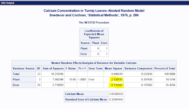
To get this:

Calculate repeatability with these highlighted numbers using is the equation from Lessells and Boag (1987); 6 is the number of samples per individual, i.e. the number of repeated measurements:
((2.520115-0.135502)/6)/(0.135502+((2.520115-0.135502)/6))
Repeatability=0.745745

To calculate measurement error, substitute 0.135502 for the current numerator (i.e. use the Bailey and Byrnes 1990 equation).
0.135502/(0.135502+((2.520115-0.135502)/6))

Measurement error=0.254255

Adding the two numbers together gets 1, which means all the variation is accounted for (and thus you only need to calculate one; to get the other just subtract from 1).

Using the ICC package's function ICCest() gives essentially the same answer (the difference appears to be the level of precision in the decimal places), but also provides confidence intervals and other data that are explained more in the Wolak et al. paper.  (Import the data first, obviously, before running this code.  You can enter it by hand or export from SAS as a .csv).

ICCest(x=plant, y=calcium, data=turnip)

>$ICC

>[1] 0.7457443

>

>$LowerCI

>[1] 0.3889918

>

>$UpperCI

>[1] 0.9776527

>

>$N

>[1] 4

>

>$k

>[1] 6

>

>$varw

>[1] 0.1355025

>

>$vara

>[1] 0.3974355

The highlighted number is repeatability, which is essentially the same as the calculation by hand from SAS barring what I believe are differences in decimal precision used in the numbers for calculating the answer.

Finally, since SAS uses a random effects model, I hoped that one might be able to calculate measurement error by hand from R just to be sure it all works.  I found a page comparing different methods of repeatability in R that showed an example using the package 'lme4'.  Calcium is the measured variable, plant is the random effect, and there are no fixed effects.

model.repeat<-lmer(calcium~1+(1|plant),
               data=turnip)
summary(model.repeat)

>results>Linear mixed model fit by REML t-tests use Satterthwaite >approximations to degrees
>  of freedom [lmerMod]
>Formula: calcium ~ 1 + (1 | plant)
>   Data: turnip
>
>REML criterion at convergence: 31.2
>
>Scaled residuals: 
>     Min       1Q   Median       3Q      Max 
>-1.09999 -0.85753 -0.09009  0.69564  2.13276 
>
>Random effects:
> Groups   Name        Variance Std.Dev.
> plant    (Intercept) 0.3974   0.6304  
> Residual             0.1355   0.3681  
>Number of obs: 24, groups:  Plant, 4
>
>Fixed effects:
>            Estimate Std. Error    df t value Pr(>|t|)   
>(Intercept)    3.012      0.324 3.000   9.295  0.00264 **
>---
>Signif. codes:  0 ‘***’ 0.001 ‘**’ 0.01 ‘*’ 0.05 ‘.’ 0.1 ‘ ’ 1

Use the residual (error, or within) as the numerator if you want to calculate measurement error, or the plant (among groups) variance as the numerator if you want to calculate repeatability.  For example, for measurement error, you get pretty close to the SAS-by-hand number.
0.1355/(0.3974+0.1355)
Measurement error=0.2542691

So, all three methods (by hand with lme4 in R, using the ICC package in R, and by hand from SAS PROC NESTED) give comparable results for the balanced design (for the plant dataset, n=6 for every individual plant, i.e. there are six measurements for any given plant).  For an unbalanced design, with varying numbers of measurements per group, Lessells and Boag (1987) provide an equation to calculate the appropriate sample size coefficient n₀ (see their equation 5).  The ICC package uses that equation to calculate n₀ (Wolak et al. 2012; this is listed as $k in the output from ICCest)  I tested this in the R packages only as I was hoping the variance from lme4 might have already been adjusted for the sample size coefficient issue.  ICC already states that they adjust (Wolak et al. 2012 and in the help file).  With the first row deleted from the turnip data set, ICC gives a repeatability value of 0.7432083 and k (which is n₀ from Lessells and Boag)= 5.73913 (slightly under the previous 6, which makes sense as I deleted one row).  With that same one-row-deleted data using lme4, I took the random effects variances (0.3952/(0.1419+0.3952)) and got 0.7358034, so its variance calculation is not including the repeatability adjustment for n₀.  This is not really surprising since that's not what it's designed to do.

So, what I will be doing to check for "measurement error" on my birds (how much "wobble" each bird has in its otherwise standard songs) is substitute the song variable (let's say frequency) for "calcium" and the bird ID (individual ID or band number) for "plant".  The random effect in lmer, the classes in SAS PROC NESTED, and x in ICCest are all the individual/subject/item from which you get repeated measurements for measurement error or repeatability.

Take home message: ICC is the easiest to use as it will take into account an unbalanced design for you already.  With SAS you can calculate for an unbalanced design but you'll have to do it by hand.  Thus, ICC and SAS should cover all cases.  With lme4 you can calculate repeatability and measurement error for balanced designs by hand, but I don't see a particularly obvious way to get the mean squares as in SAS (and I need to move on to other parts for the analysis), so I'm going to leave it at that for now.

Here are the papers I used to understand how to calculate measurement error and repeatability:
Bailey RC, Byrnes J. 1990. A new, old method for assessing measurement error in both univariate and multivariate morphometric studies. Systematic Biology 39:124–130.

Lessells CM, Boag PT. 1987. Unrepeatable repeatabilities: a common mistake. Auk 104:116–121.
Wolak ME, Fairbairn DJ, Paulsen YR. 2012. Guidelines for estimating repeatability.  Methods in Ecology and Evolution 3:129-137.

and here are some helpful examples of papers that use measurement error:
Lougheed SC, Arnold TW, Bailey RC. 1991. Measurement error of external and skeletal variables in birds and its effect on principal components. Auk 108:432–436.
Marantz CA, Patten MA. 2010. Quantifying subspecies analysis: a case study of morphometric variation and subspecies in the woodcreeper genus Dendrocolaptes. Ornithological Monographs 67:123–140.

A belated Happy New Year from the frozen north

May all the snow you eat be tasty and fresh.  10 January 2016, Winnipeg, MB, Canada.